PowerExpect

Posted on October 13, 2025 • 26 min read • 5,468 words

Power Markets Time Series Forecasting Machine Learning/Deep Learning

Share via

Link copied to clipboard

A fast and simple app for viewing forecast and actual electricity prices for French and German/Luxembourg bidding zones.

Open App

Click here

1. Motivation

The initial goal of this project was twofold: on the one hand, to learn a framework specialized in frontend development, and on the other hand, to test new methods/architectures for time series forecasting applied to electricity price forecasting.

Python frontend libraries are often limited and/or slow. I therefore wanted to test a framework specialized in frontend development for web applications. I chose Vue.js, which seemed to be the most accessible option.

I also wanted a comprehensive tool that would allow me to easily test new methods and models for time series forecasting, particularly electricity price forecasting, in real-world conditions. When working on this type of project in industry, you generally prefer to use what you know already works well, following Occam’s razor and under time constraints. This often leaves little room for in-depth exploration of new things. However, there is a wealth of literature on the subject, making me very curious.

2. Introduction

Electricity Price Forecasting (EPF) is a well-known application of Time Series Forecasting (TSF) methods. This question has been explored for over 30 years now, since the wave of electricity market liberalisation in the 1990s, and is attracting increasing interest in the literature [1]. Firstly because TSF itself is attracting growing interest [2] and secondly because EPF plays a fundamental role in energy markets, enabling market players to optimize their trading strategies, reduce financial risks, and maintain grid stability [3]. However, this is a complex (and increasingly so) exercise because short-term price fluctuations are highly sensitive to renewable energy generation forecasts, regulatory and geopolitical announcements, and unforeseen disruptions such as generation outages or grid constraints. This results in prices with high volatility, non-linearity, and sudden spikes [3]. There are several EPF methods, but only those involving Machine Learning (ML) are of interest here.

The history of EPF has closely followed the history of TSF. TSF began with statistical methods based on moving averages developed in the 1950s to 1970s (exponential smoothing/ARIMA). It then continued with the first ML methods such as decision trees in the 1980s, followed by GBM (Gradient Boosting Machines) in 1999/2001. At the same time, deep learning (DL) models appeared with RNNs and LSTMs in the 1990s [2].

These fundamental building blocks were subsequently expanded, improved, and combined to create the wide variety of architectures we have today. Popular implementations of GBM such as XGBoost and LightGBM, which were not specifically designed for time series forecasting, appeared in the 2010s and quickly became standards in the field thanks to their performance and interpretability. Deep learning models have received increasing interest, with architectures based on MLP (Multi-Layer Perceptron) such as NBEATS and TIDE, and transformer-based architectures such as PatchTST and PETformer. Following the rise of foundation models for natural language processing, foundation models for time series forecasting have emerged, such as TimeGPT and Lag-Llama. Advances have also been made in other architectures, such as Mamba models, and in related areas such as feature engineering. Overall, TSF is a particularly dynamic and fruitful area of research, where many ideas show great potential [2].

The aim of EPF (and more generally of TSF) is to find a sufficient approximation according to certain metrics of the function:

f : Z = \Big(\pmb{y}_{t-L+1:t},\;\pmb{X}^{(n)}_{t-L+1:t},\;\pmb{X}^{(m)}_{t+1:t+H}\Big) \longmapsto f(Z) = \pmb{\hat{y}}_{t+1:t+H}

With:

$L$ = The past observations window size
$H$ = Forecast horizon
$n$ = Number of features
$m$ = Number of features available during forecast ( $m \le n$ )
$\pmb{y}_{t-L+1:t} \in \mathbb{R}^{\,L}$ = Vector of $L$ past observations
$\pmb{X}^{(n)}_{t-L+1:t} \in \mathbb{R}^{\,L \times n}$ = The matrix of $n$ explanatory variables over $L$ time steps
$\pmb{X}^{(m)}_{t+1:t+H} \in \mathbb{R}^{\,H \times m}$ = The matrix of $m$ features over $H$
$\pmb{\hat{y}}_{t+1:t+H} \in \mathbb{R}^{\,H}$ = The vector of the target variable forecast over $H$

The choice of $f$ is an architectural choice. It is based on several factors, such as our knowledge of the field of application, our belief in the architecture’s ability to model the relationships between the features and the target variable for this problem, and our understanding of the literature.

In this project, the choice of $f$ is based primarily on my curiosity after reading a paper on EPF or TSF.

3. Workflow

The PowerExpect application has its backend on AWS and its frontend on Vercel. I wanted to have for this project an application that updates automatically every day, following the pace of day-ahead auctions. This meant I needed a machine that would launch every day, execute the code, and then save the results in a storage location accessible via an API by the frontend. I chose AWS, which I was already familiar with. The CI/CD pipeline is handled by CodePipeline and Codebuild, which automatically retrieve the code from my GitHub repository, then build the Docker image and store it in ECR. An EC2 instance is launched every day via a lambda controlled by EventBridge. The instance retrieves the image from ECR when it starts up and executes it. All updated inputs and outputs are saved in two separate private S3 buckets. The logs are also sent to my email address by the instance so that I don’t have to log in to AWS every time, which is a bit of a pain with MFA. The files on S3 can be large and exceed Amazon’s service limit. So I opted to download them directly to S3 from the frontend via 1-second pre-signed URLs served by an API.

4. Data

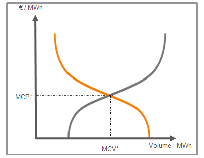
The day-ahead (or SPOT) price for each 15 minutes of the following day is determined by an auction for each market in Europe. There are therefore 96 auctions for the French zone and for the German zone. Participants have until noon to indicate the volumes they want to buy/sell based on the price. The price at time t will therefore be the intersection between the aggregate demand curves at t and the supply curves at t for each participant [4].

SPOT prices are therefore driven by supply (generation) and demand (consumption), which are themselves driven by numerous factors. The structure of the market in question, the composition of the electricity mix, the weather, balancing markets, operational constraints, the availability of power plants, seasonality/calendar (time, day, season, etc.), fuel prices, and CO2 quota prices all influence supply. Similarly, demand is influenced by seasonality/calendar and temperature effects, but also by other factors such as consumption habits [5].

CAL+1 prices, i.e. the series of prices for calendar contracts traded daily on exchanges in year Y for delivery in year Y+1, are currently being added.

Like any time series, prices are strongly correlated with previous values. An autocorrelation and partial correlation study on both markets makes it easy to select relevant lags. I have chosen lags common to both markets to simplify the pipelines.

For the time being, only the main and easily available influencing factors, such as generation and total demand, are used in order to limit the complexity of the models. Inevitably, this also limits their predictive power.

Data is primarily sourced from the great ENTSOE Transparency Platform . This data is accessible free of charge via an API. Models are trained on post-energy crisis data from 2022. The forecast horizon is currently one day, or 96 points.

5. NHITS

a. Architecture

N-HiTS, which stands for “Neural Hierarchical Interpolation for Time Series” [6], falls into the category of MLP-based DL architectures, which have now proven to be among the best options available. This model was introduced to overcome two typical problems in long-term forecasting: complexity, i.e. memory costs that explode with the size of the horizon, and forecast volatility, i.e. the difficulty of obtaining reliable and stable long-term forecasts.

To do this, the researchers started with the NBEATS model introduced three years earlier [7] and then improved it using two techniques: “Multi-rate Signal Sampling” and “Hierarchical Interpolation” [6].

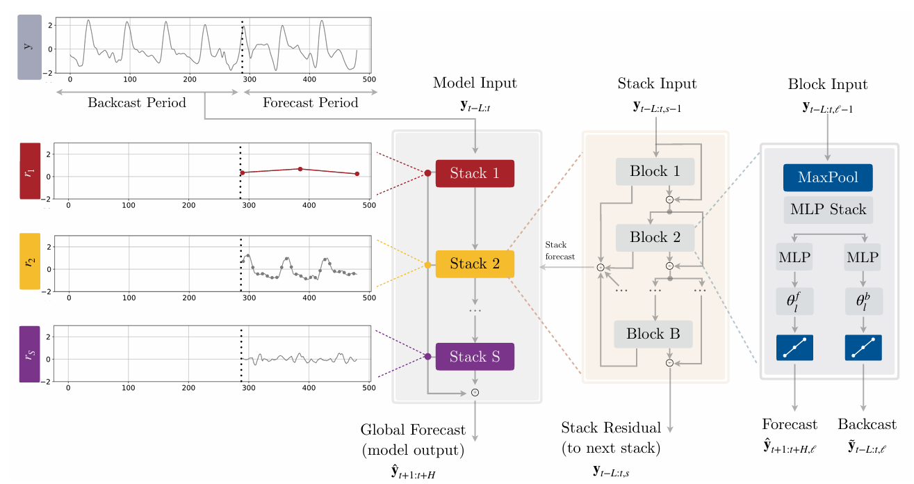
The figure above illustrates the univariate version of the N-HiTS architecture, which simplifies the equation of the problem posed in the introduction but is sufficient to understand how the model works (see NBEATSx for more information on incorporating exogenous variables into the architecture [8]). Thus, this version only takes as input the vector of past observations, denoted here as $\pmb{y}_{t-L:t}$ with $L$ being the number of lags. We can see that N-HiTS is based on a 3-layer architecture with S stacks, each composed of B blocks. The highest level layer corresponds to the overview with the arrangement of stacks, the next to the arrangement of blocks within each stack, and the last to the components within each block [6].

1st layer

N-HiTS is composed of S stacks, each of which models different frequencies of the time series. A stack takes as input the residual of the previous stack $\pmb{y}_{t-L:t,s-1}$ (except for the first stack of course, which takes $\pmb{y}_{t-L:t}$ directly) and returns its forecast $\pmb{\hat{y}}_{t+1:t+H,s}$ and its residual $\pmb{y}_{t-L:t,s}$ . The forecasts of each stack are added together to form the final forecast (the model also returns the residual of the last stack S $\pmb{y}_{t-L:t,S}$ ) [6]:

\pmb{\hat{y}}_{t+1:t+H} = \sum_{s=1}^S \pmb{\hat{y}}_{t+1:t+H,s}

2nd layer

Similar to stacks (and comparable to boosting models), the B blocks of a stack s are assembled hierarchically, where the input of block $l$ is the residual of block $l-1$ . In fact, the backcast output of a block $l$ denoted $\pmb{\tilde{y}}_{t-L:t,l}$ is used to clean the input $\pmb{y}_{t-L:t,l+1}$ of the next block. This allows the blocks to focus their attention on parts of the series that are not understood. The forecasts of each block are added together to form the final forecast of the stack [6]:

\pmb{y}_{t-L:t,l+1} = \pmb{y}_{t-L:t,l} - \pmb{\tilde{y}}_{t-L:t,l}

\pmb{\hat{y}}_{t+1:t+H,s} = \sum_{l=1}^B \pmb{\hat{y}}_{t+1:t+H,l}

3rd layer

Each block begins with a max pooling layer with filter size $k_l$ followed by an MLP. The pooling step allows the block to focus on a specific frequency of the input series. A large $k_l$ will filter out high frequencies, forcing the MLP to model a low-frequency series, and conversely, a small $k_l$ will force the MLP to model a high-frequency series. This is called “multi-rate signal sampling”. This step has two advantages: First, it allows the model to focus on low-frequency aspects of the time series, which produces more stable and consistent long-term forecasts. Second, it reduces the size of the MLP input, thereby decreasing the complexity of the calculation (and thus improving training speed) and the risk of overfitting. With $\pmb{y}_{t-L:t,l}$ as the input vector of block $l$ , we have [6]:

\pmb{y}^{(p)}_{t-L:t,l} = MaxPool(\pmb{y}_{t-L:t,l}, k_l)

~

Block $l$ will then use the reduced input to estimate the backward interpolation parameters ${\theta}^b_l$ and forward interpolation parameters ${\theta}^f_l$ by estimating the hidden vector $h_b$ with an MLP and then projecting it linearly [6]:

h_l = MLP_l(\pmb{y}^{(p)}_{t-L:t,l})

{\theta}^f_l = LINEAR^f(h_l)

{\theta}^b_l = LINEAR^b(h_l)

~

Finally, the output vectors of block $l$ $\pmb{\tilde{y}}_{t-L:t,l}$ and $\pmb{\hat{y}}_{t+1:t+H,l}$ are computed by “hierarchical interpolation” [6].

Once the coefficients ${\theta}^b_l$ and ${\theta}^f_l$ have been computed, it is necessary to restore the initial sampling rate or granularity (modified by the max pooling/multi-rate signal sampling operation) in order to predict all H points in the forecast horizon. To do this, N-HiTS performs “temporal interpolation” using the interpolation function $g$ [6]:

\forall \tau \in \{t+1, \dots, t+H\}, ~\hat{y}_{\tau,l} = g(\tau,{\theta}^f_l)

\forall \tau \in \{t-L, \dots, t\}, ~\tilde{y}_{\tau,l} = g(\tau,{\theta}^b_l)

~

$g$ can take the form of a nearest neighbor function, piecewise linear, or cubic. The authors of N-HiTS indicate that, on average across all tested datasets, prediction accuracy and computational performance favor the linear method, where $g$ is expressed as [6]:

g(\tau,\theta) = \theta [t_1] + (\frac{\theta [t_2] - \theta [t_1]}{t_2 - t_1}(\tau - t_1))

With:

$t_2 = t_1 + 1/r_l$
$t_1 = argmin_{t \in T:t\leq \tau} (\tau - t)$

The time partition $T$ used to calculate $t_1$ is defined as $T = \{t + 1, t + 1 + 1/r_l, \dots, t + H − 1/r_l, t + H\}$ where $r_l$ is called the “expressivity ratio” and controls the number of parameters per unit of output time: $|\theta^f_l| = ⌈r_l H⌉$ (smallest integer greater than or equal to $r_l H$ ). Using this ratio and temporal interpolation avoids the explosion in memory cost and computational complexity that occurs as the horizon increases, a recurring problem in other architectures such as transformers.

N-HiTS will force the expressivity ratio $r_l$ to synchronize with the size of the filter $k_l$ used in multi-rate signal sampling, and this is where the power of the architecture lies. Considering a top-down approach (which proves to be more effective than a bottom-up approach on the datasets tested in the paper), i.e. by choosing increasing $r_l$ and therefore decreasing $k_l$ , the blocks will learn both to observe and generate signals with increasingly fine granularity/frequency. This approach, which prioritizes the specialization of each block and therefore each stack in a specific frequency, is called “hierarchical interpolation”. By cleverly choosing the $r_l$ , we can match the frequency of the blocks with known cycles in the time series, such as months, weeks, days, etc [6].

In short, N-HiTS is a generalization of N-BEATS that offers accurate, interpretable, stable forecasts across all horizons, while minimizing memory costs and training time. N-HiTS greatly enhances the power of MLP-based architectures.

With the recent switch in October 2025 from hourly to 15-minute intervals for European day-ahead markets, thereby multiplying the forecasting horizon by 4, the use of models designed for long-term forecasting such as N-HiTS has undoubtedly become more relevant.

b. Hyperparameters

Hyperparameters are fine-tuned using the tree-structured Parzen estimator (TPE) approach [9] implemented in hyperopt (see section “built with”).

c. Training

6. HSL

a. Architecture

Hybrid or ensemble models, which combine several models and methods, are a solid choice for EPF/TSF [3]. They are particularly effective at capturing the complex, nonlinear, and volatile dynamics of electricity markets by leveraging the strengths of multiple architectures. The paper presenting the following model provides an example of combination that can be used specifically for EPF [10].

HSL stands for “Hybrid Stacking Lasso” and is a hybrid model combining six base models: XGBoost, CatBoost, LightGBM, LSTM, GRU, and NODE. These basic models are combined by stacking, using Lasso regression as the meta-model [10].

Each base model has its strengths: XGBoost is robust on structured data and has a good ability to capture nonlinear interactions. LightGBM is effective on large datasets, enabling fast training and good temporal feature extraction. CatBoost performs well in its handling of categorical variables and its resistance to overfitting. LSTM and GRU are included for their ability to model long-term temporal patterns. NODE, by combining decision trees and neural networks, can capture complex and nonlinear interactions on tabular data [10].

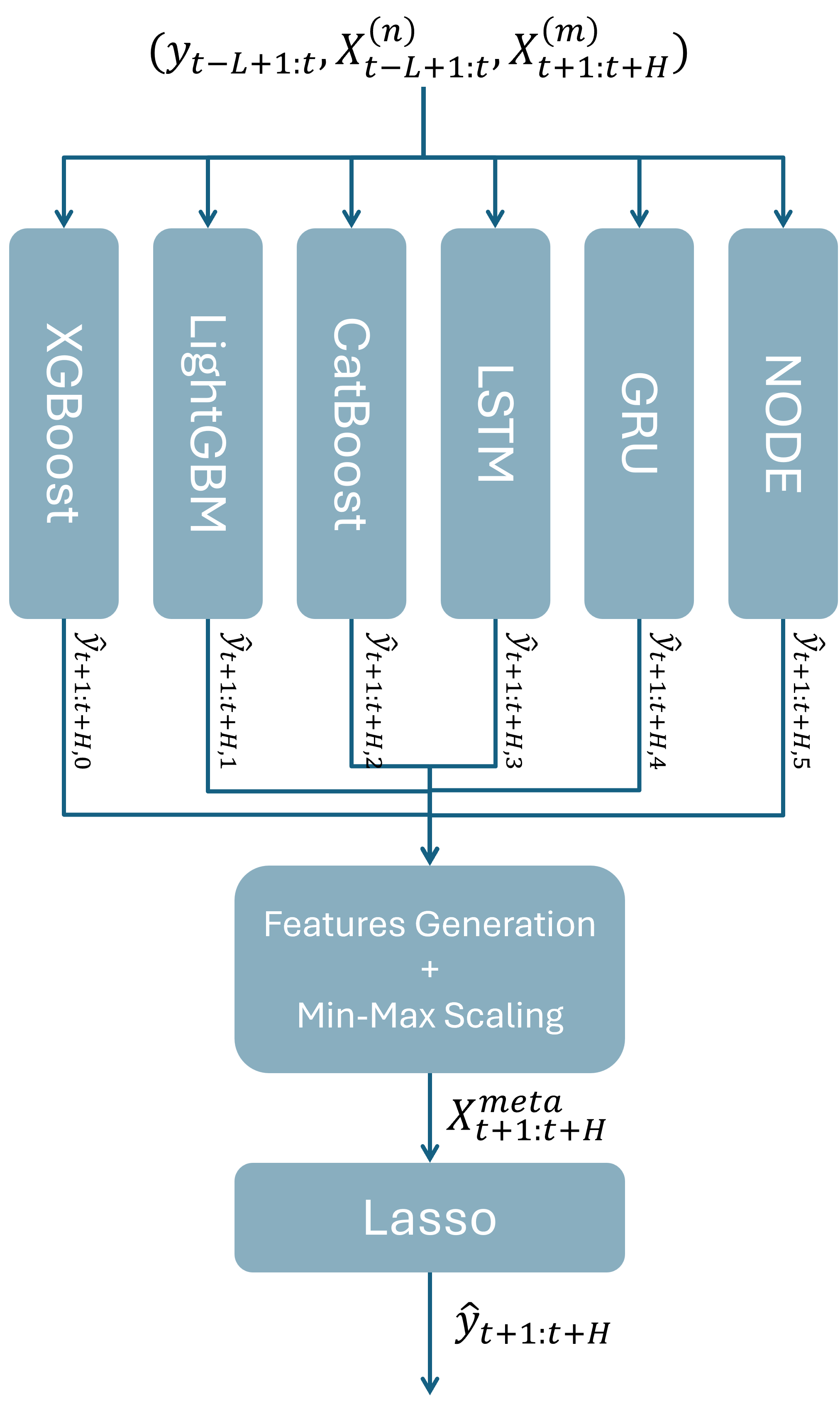
The forecasts of each base model are concatenated and then normalized to $[0,1]$ using Min-Max scaling:

\forall i \in \{0,\dots,5\}, ~\hat{y}^{scaled}_{t+1:t+H,i} = \frac{\hat{y}_{t+1:t+H,i} - min(\hat{y}_{t+1:t+H,i})}{max(\hat{y}_{t+1:t+H,i}) - min(\hat{y}_{t+1:t+H,i})}

$~$

Next, the matrix with the scaled forecasts is augmented with temporal variables (hours, days, weeks, etc.) to form the meta-feature matrix $X^{meta}_{t+1:t+H}$ used as input for the meta-model. The article introducing HSL does not provide any information on the strategies to be used to train the meta-model. This leaves us free to test different things while respecting the philosophy of the original paper. I therefore followed some of the recommendations in Jason Brownlee’s cool article on stacking algorithms [11]. For example, he points out that adding other explanatory variables to the meta-model can provide it with additional context on the best way to combine the forecasts from the base models. Tests confirmed this approach. Furthermore, increasing the input size is not a concern when using Lasso regression as a meta-learner, since unnecessary variables will be dropped. The final forecast is written as:

\hat{y}_{t+1:t+H} = X^{meta}_{t+1:t+H}.W

~

With $W$ the weight vector of dimension H. This vector is found by minimizing the objective function $J$ over the training period $\tau$ where the Lasso term appears:

J(W) = L(y_{\tau}, \hat{y}_{\tau}) + \alpha||W||_1

With:

$L$ the loss function
$\alpha$ the regularisation parameter
$||W||_1 = \sum_i |w_i|$ L1 norm applied to model weights

Lasso/L1 regularization sets weights to zero in directions where the cost function is not sensitive. Thus, it attempts to set parameters that are not very important to zero, which makes it possible to handle large input matrices and promotes a minimalist solution. Let’s now describe each base model in detail.

b. XGBoost

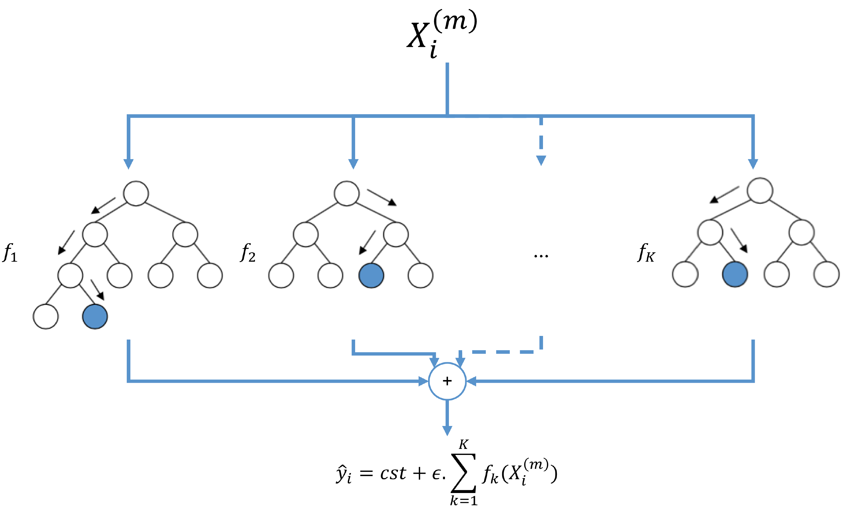
Architecture Gradient Boosting Machine/Tree

XGBoost, which stands for “Extreme Gradient Boosting”, is a machine learning architecture based on the GBMs mentioned in the introduction and developed at the beginning of the century. It is an ensemble model that uses CARTs (“Classification And Regression Trees”) called “weak learners” as base models. CARTs are similar to simple decision trees, except that a score is associated with each of the leaves/nodes, allowing them to handle regression problems with continuous variables.

As a reminder, a decision tree is a non-parametric (=there are no underlying assumptions about the distribution of errors or data and the model is based simply on the observed data) supervised learning method. They can be used to predict the value of a target variable by learning simple decision rules inferred from the data features. They are highly interpretable as they directly and visually illustrate the decision-making process. This interpretability is lost with most ensemble methods.

XGBoost combines trees through boosting, where the model’s forecast is equal to the sum of each tree’s forecast for each time step [12]:

\forall i \in \{t+1, \dots, t+H\}, ~\hat{y}_{i} = cst + \epsilon\sum^K_{k=1} f_k(X^{(m)}_{i})

With:

$K$ = the number of trees.
$f_k$ = the structure of the k-th regression tree.
$X^{(m)}_{i}$ = the vector of the $m$ features at index $i$ .
$\epsilon$ = the learning rate. The larger it is, the more trees will need to generalise in order to predict the residual, thus preventing overfitting.
$cst$ = the default forecast if the model didn’t have trees.

The functions $f_1$ to $f_K$ are learnt by boosting, adding one tree after another. Hence [12]:

\forall k \in \{1, \dots, K\}, \forall i \in \{1, \dots, n\},~\hat{y}^{(k)}_{i} = \hat{y}^{(k-1)}_{i} + \epsilon.f_k(X^{(m)}_{i})

~

Thus, the model will grow as trees are added, and each tree will learn to predict the residual of the previous tree. The objective function to be minimised in order to train the k-th tree is written as [12]:

J^{(k)} = \sum_{i=1}^n l(y_i, \hat{y}^{(k)}_i) + \Omega (f_k) = \sum_{i=1}^n l(y_i, \hat{y}^{(k-1)}_i + \epsilon.f_k(X^{(m)}_{i})) + \Omega (f_k)

With:

$l$ the loss function.
$\Omega$ the regularisation function.

Let $w \in \mathbb{R}^T$ be the vector of weights for each leaf $j \in \{1, \dots, T\}$ (where $T$ = number of leaves in the k-th tree) and $q: \mathbb{R}^m \longrightarrow\ \{1, \dots, T\}$ the tree structure that associates the features to a leaf $j$ . We have: $f_k(X) = w_{q(X)}$ [12].

Furthermore, by considering ridge regularisation plus a term $\gamma T$ to encourage simple trees, we can write:

\Omega (f_k) = \gamma T + \frac{1}{2} \lambda \sum^T_{j=1} w_j^2

~

$\lambda$ reduces the sensitivity of the weights $w_j$ to the observed values which limits overfitting.

Thus, by approximating $J^{(k)}$ using a second-order Taylor expansion and simplifying (= removing the sum of losses, which is a constant, and setting $\epsilon = 1$ ), we get [12]:

\tilde{J}^{(k)} = \sum^T_{j=1} [w_j \sum_{i \in I_j} g_i^{(k)} + \frac{1}{2} (\sum_{i \in I_j} h_i^{(k)} + \lambda)w_j^2] + \gamma T

With:

$I_j = \{i | q(X^{(m)}_{i})=j \}$ the set of indices of the $m$ features associated with the j-th leaf.
$g_i^{(k)} = \partial_{\hat{y}^{(k-1)}_i} l(y_i, \hat{y}^{(k-1)}_i)$ the i-th first-order gradient of the k-th tree or boosting iteration.
$h_i^{(k)} = \partial^2_{\hat{y}^{(k-1)}_i} l(y_i, \hat{y}^{(k-1)}_i)$ the i-th second-order gradient of the k-th boosting iteration.

For a given structure $q$ , the optimal weight of the j-th leaf $w_j^*$ is then written as [12]:

w_j^* = \frac{\sum_{i \in I_j} g_i^{(k)}}{\sum_{i \in I_j} h_i^{(k)} + \lambda}

And the optimal value $\tilde{J}^{(k)^*}(q)$ :

\tilde{J}^{(k)^*}(q) = -\frac{1}{2}\sum^T_{j=1}\underbrace{\frac{(\sum_{i \in I_j} g_i^{(k)})^2}{\sum_{i \in I_j} h_i^{(k)} + \lambda}}_{cost~of~the~j~th~leaf} + \gamma T

The cost $\tilde{J}^{(k)^*}(q)$ measures the performance of the tree structure $q$ by comparing the regularisation term on the number of leaves to the cost of each leaf. The smaller $\tilde{J}^{(k)^*}(q)$ is, the better the tree structure performs [12].

If we used the mean square error as the loss function, then we would have $g_i^{(k)} = \hat{y}^{(k-1)}_i - y_i$ et $h_i^{(k)} = 1$ . So:

w_j^* = \frac{\sum_{i \in I_j} (\hat{y}^{(k-1)}_i - y_i)}{|I_j| + \lambda} = \frac{sum~of~residuals~from~previous~tree}{number~of~residuals + \lambda}

and:

\tilde{J}^{(k)^*}(q) = -\frac{1}{2}\sum^T_{j=1}\underbrace{\frac{(\sum_{i \in I_j} (\hat{y}^{(k-1)}_i - y_i))^2}{|I_j| + \lambda}}_{cost~of~the~j~th~leaf} + \gamma T = -\frac{1}{2}\sum^T_{j=1}\frac{squared~sum~of~residuals~from~previous~tree}{number~of~residuals + \lambda} + \gamma T

~

Now, we need to test every possible structure, i.e. every possible split combination (= one parent or root node and two child leaves), and keep the one that offers the best performance (= smallest possible $\tilde{J}^{(k)^*}(q)$ ). This search is costly in terms of complexity and potentially also in terms of memory, since the costs of each possible leaf and therefore their gradients ( $o(T.m.(n-1))$ ) must be computed.

XGBoost’s first approach is to use an exact algorithm (“Exact Greedy Algorithm”) that starts from a leaf and iteratively adds the branches of the best splits. It runs through all the sorted values of the features and accumulates the gradients, which allows it to lower the memory cost. To select the best split, the algorithm will choose the one that maximises the following score [12]:

score_{split} = \frac{1}{2}[cost~of~the~left~leaf + cost~of~the~right~leaf - cost~of~the~root] - \gamma

~

The higher the score, the more the split lowers the cost of the tree.

Once the structure has been built, XGBoost will optimise it by removing splits that have a negative score. This tree pruning is controlled by the regularisation parameter $\gamma$ , which reflects a greater or lesser desire to have deep trees, i.e. a complex solution that is likely to overfit [12]. Other parameters can be used to manage the complexity of the model, such as max_depth, which limits the maximum depth of the trees.

Usually, XGBoost will use variants of the exact algorithm to find splits in a more optimised way. This is because the exact algorithm is computationally expensive and difficult to scale, as it tests all possible splits. For example, if the input data is too large, XGBoost will use an algorithm (“Approximate Algorithm”) that reduces the number of splits tested to well-chosen percentiles [12].

In summary, XGBoost will make a forecast by summing the forecasts of each tree for each time step. During training, the model is built by adding trees one after the other in a cumulative way. Each tree is built by starting with a root and then adding other leaves level by level. Leaf splits are chosen to maximise a score that represents the leaf’s contribution to error reduction. XGBoost uses different regularisation terms to avoid overfitting and limit model complexity, such as $\gamma$ , a threshold below which the split is considered to contribute enough to error reduction.

As XGBoost is based on trees where specific features are chosen for its splits, we can deduce the weight of each of them in the foercast, which makes the model easier to interpret than other methods such as those based on neural networks. In addition to the founding paper [12], I recommend the video series from statquest for more details on XGBoost.

c. LightGBM

LightGBM, which stands for “Light Gradient Boosting Machine”, offers an optimised implementation of GBM similar to XGBoost (see previous section). This algorithm takes performance optimisation further than XGBoost by introducing two improvements called “Gradient-based One-Side Sampling” (GOSS) and “Exclusive Feature Bundling” (EFB) [13].

The challenge with GBM implementations is always the same: how to optimise split finding while maintaining maximum performance ? The natural approach is to reduce the number of candidate splits (by reducing the number of splits to be tested or by resampling the amount of observed data) and features tested. LightGBM uses the GOSS algorithm, which keeps all data with significant gradients (above a predefined threshold) and performs random sampling on data with low gradients. In addition to GOSS, LightGBM introduces the EFB algorithm, which groups certain features together, thereby reducing the search space for splits [13].

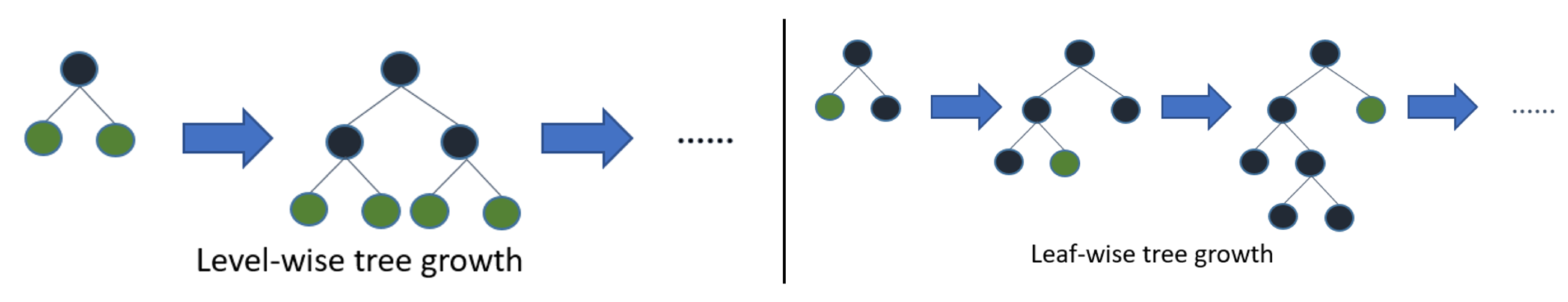
Another important feature of LightGBM is the way it builds its trees. Unlike other implementations such as XGBoost, which do so level by level, LightGBM builds its trees leaf by leaf, choosing (according to a criterion) the best next leaf to process. With an equal number of leaves, this approach tends to yield better results. See the library documentation (built with section) for more information on this subject [13].

d. CatBoost

CatBoost for “Categorical Boosting” is, like XGBoost and LightGBM, an implementation of a GBM (see the XGBoost section for notations). CatBoost stands out for its handling of categorical variables and its approach to boosting to solve target leakages [14].

Categorical Features

A categorical feature consists of a discrete set of distinct values called categories. For example in TSF, we sometimes consider times of day (morning, afternoon, evening, etc.). These categorical variables can provide a substantial gain in information. However, they require a crucial encoding step, i.e. transforming the categories into numerical values that can be understood by the model with minimal loss of information [14].

There are several methods for encoding categorical features . A classic encoding method is “one-hot encoding”, which consists of converting each category into a binary column vector (1 for indices where the category appears and 0 otherwise). Obviously, this method is quickly limited by the number of categories to be encoded. Another popular method is “target encoding”, which consists of replacing categories with statistical values of the target variable. For example, we can use the average of the target variable values for each category. This simple approach should be avoided, as it will lead to data leakage: the test data will contain information from the training data. Several methods are possible to solve this problem, such as partitioning the training data [14].

CatBoost uses a target encoding strategy described as more effective by the founding paper. Simply put, CatBoost encodes categories based solely on previously observed values. This means that CatBoost applies category encoding sequentially, thus avoiding any target leakage. Since the order of the categories is important, this approach is called “ordered target statistics” or “ordered target encoding”. The numerical value of the category will then be calculated as the average of past observations for that category, smoothed by a constant $p$ (=prior) such that the value of category $k$ at index $i$ is written as [14]:

x_i^k=\frac{\sum_{j\in I_i^k}y_j + p}{|I_i^k| + 1}

~

With $I_i^k$ the set of indices preceding the index $i$ where $y$ is 1 for category $k$ (when the target is continuous, we simply use statistical intervals/bins).

During inference, the categories are encoded by taking all the previously encoded values.

Ordered Boosting

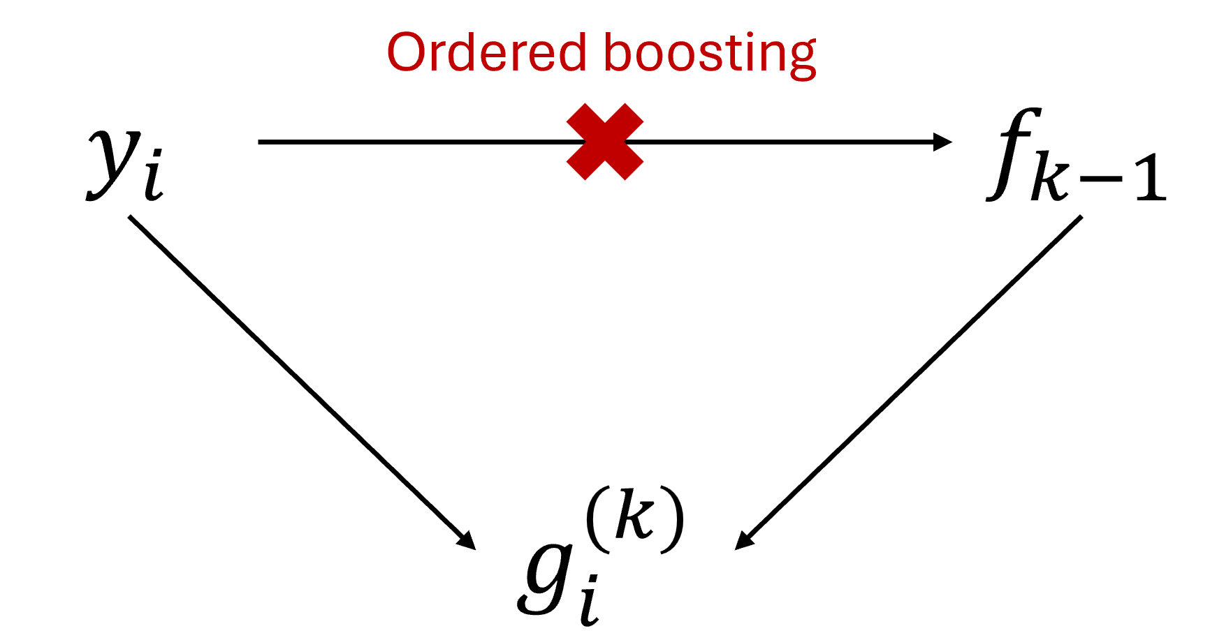
Just like ordered encoding for processing categorical variables, ordered boosting is motivated by the presence of target leakage during training. Indeed, the authors of the original CatBoost paper show that in a simple case where the same dataset is used to train each tree, a bias inversely proportional to the size of the dataset shifts the prediction. This stems from the use of the same target variables for gradient estimation and tree training. Indeed, we compute the $g_i^{(k)}$ using the target $y_i$ and the prediction $f_{k-1}(x_i,y_i)$ , whereas the tree $f_{k-1}$ was itself built using $y_i$ . This is a target leakage that causes a shift in the conditional distribution of the gradients $g_i^{(k)}(x_i,y_i) |x_i$ (and therefore $f_k(x_i,y_i)|x_i$ ) relative to that on the test data and ultimately leads to a biased prediction and a model that generalises less well. To solve this, CatBoost uses ordered boosting [14].

Ordered boosting suggests to solve the leakage issue by using previous examples $(x_{0:i-1},y_{0:i-1})$ to train $f_{k-1}$ . Thus, $f_{k-1}(x_i,y_i)$ has never seen the example $(x_i,y_i)$ and the $g_i^{(k)}$ will not be estimated with a biased $f_{k-1}$ . This approach is the same as the one used for ordered encoding by processing the data sequentially, row by row [14].

The naive or brute force implementation of ordered boosting would consist of training n (=number of examples/observations, $i \in \{1, \dots, n\}$ ) models $M_1, \dots, M_n$ , such that model $M_i$ is trained only on the i-th observations of a random permutation of the data set. Then, model $M_{i-1}$ is used to calculate $g_i$ . However, this naive solution is too complex: training n models would be too costly in terms of time and memory. To reduce the complexity of the implementation and use ordered boosting, CatBoost proceeds as follows [14].

First, CatBoost generates a set of random permutations of the data set, on which to perform ordered encoding and then train each tree. Thus, the gradients $g_i^{(k)}$ and categorical variables will be calculated using a different history at each boosting step $k$ . This still ensures that no model has seen the example for which the gradient is calculated, but reduces instability due to the fact that an example at the beginning of the permutation would have very little previous data [14].

Next, CatBoost trains its weak learners, which are symmetric or oblivious decision trees, i.e. trees in which all leaves at a level have the same split/division criterion. These trees are less prone to overfitting and significantly speed up execution at test time. The trees are trained sequentially, where the gradient $g_i$ is calculated using the prediction $M_{r,j}(i)$ of the i-th example using the first j-th examples of permutation r. In practice, instead of keeping all predictions $M_{r,j}(i)$ , CatBoost only keeps intermediate predictions at geometric intervals (at indices $2^k$ ). This is possible thanks to the symmetric structure of the trees. Thus, if there are s permutations, then the complexity of updating the models $M_{r,j}$ and computing the gradients goes from $O(sn^2)$ to $O(sn)$ [14].